CUDA Pathtracer
Contents
- Introduction to Pathtracing
- Pathtracer Implementation
- Visual Effects
- Performance Improvements
- Bloopers
- Acknowledgements
Introduction to Pathtracing
Starting this project, I had minimal knowledge of pathtracing. All I knew is that it was somewhat related to raytracing and I knew it was a Big Deal for games. If you’re familiar with pathtracing/raytracing, feel free to skip ahead to my project details. Otherwise I’ll talk a bit about pathtracing and how it works in general.
Rendering is hard. There are a lot of materials in the world. Creating a realistic representation through traditional rendering can be tedious and, in the end, doesn’t look that great. PPathtracing provides a more realistic rendered image by simulating the laws of physics. Simply, a number of rays are generated on a point representing our camera. Each ray is then sent out in in each direction from the point. For each ray, the pathtracer calculates where it will intersect from its current position and direction and then calculates where its going next. This is done with the help of our shaders. The shaders determine not only the color of the bounced ray, but in what direction it is going. This is where the physical properties of the material come into play.
Each object in the scene can be Reflective, Refractive, Diffuse, or proportion of the three. The ratios and properties of each material are used when rendering to more accurately simulate the light-material interactions we would see in the real world. When light interacts with a diffuse object (think chalkboard) it can bounce in any direction. This creates a rough, plain looking surface. Reflective materials (think a mirror or a chrome fender) bounce rays in a generally consistent direction. Perfectly reflective materials are more likely to bounce it in a particular direction, while less reflective materials will have a bit more divergence. Refractive materials (think water) will allow most light to pass through, but the path of the light will change. I talk more about the physics of each further down.
The pathtracer looks at each intersection between a ray and a material and picks one of the properties to apply, and if enough rays are used enough times, this averages out to look pretty realistic. The pathtracer will generate rays from a camera, bounce them around the scene a couple times, and then repeat this process. Over many samples, the image starts to converge and look good. There are some problems with sampling this way, but as we’ll see in a bit the pathtracer can add noise to each sample to create small differences in the initial rays for each sample. This creates a smoother image and tries to hide some of the imperfections of digital rendering.
Pathtracer Implementation
The base pathtracer given to me had functions to read in scene descriptions, fire off rays, and do minimal shading. I implemented additional shaders and features to improve the quality and capabilities of the renderer. I’ve split this into two groups, visual improvements and performance improvements.
Visual Improvements
- Ideal Diffuse Scattering Function
- Imperfect Specular Reflective Scattering Function
- Refractive Transmission Scattering Function using Fresnel Effects and Shlick’s Approximation
- Antialiasing with Stochastic Sampling
- Depth of Field
- Motion Blur Effects
- Loading of glTF Object Files (Partial)
Performance Improvements
- Compaction of Terminated Rays
- First-Bounce Caching
- Material Sorting for Memory coherence
In the following sections I’ll discuss each objects implementation and its effects.
Ideal Diffuse Scattering Function
This was mostly a freebie so I will not go into it in too much detail. When a ray intersects a non-specular object, it will bounce the incoming ray in a random direction in a hemisphere about the normal. This is done by taking a random θ and ψ around the normal and mapping it to cartesian coordinates.
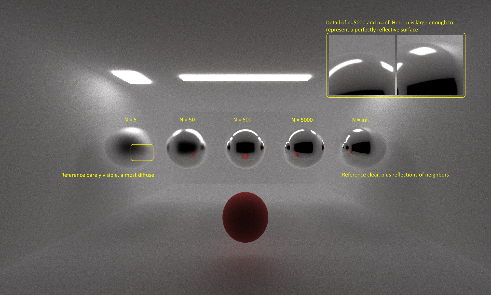
Imperfect Specular Reflective Scattering Function
Reflective materials have a ‘shininess’ property that changes how reflective they are. A mirror, for example, is nearly perfectly reflective. A chrome bumper on a car may be less reflective, and a small marbles even less so. This is represented in the pathtracer by using importance sampling. A perfectly reflective object (shininess → ∞) will always bounce a ray at θi = θo. However, for smaller shininess values, the ray will bounce in some distribution centered on the perfectly reflected ray. My renderer determines this by taking n = shininess, R = 𝒰[0,1), and ψo = acos(R1 / n + 1) and θo = 2πR. I then take these values, transform them to the proper coordinates, and then transform it to be centered on the normal. Observe that for infinite n, ψo will be 0o, so there would be no change from the perfectly reflected angle.
Refractive Transmission Scattering Function
Refraction is a bit trickier from the above two because of a couple of unique properties. First of all, there is the case of total internal reflection. After a certain critical angle θc, the ray will not transmit through the material and it will simply reflect off of the surface (internal or external). This can be seen in the real world by looking out on the ocean during a sunset. Light from the sun will mostly bounce off the surface of the water to your eyes. High indices of refraction η will lead to greater distortion of the rays moving through the medium.
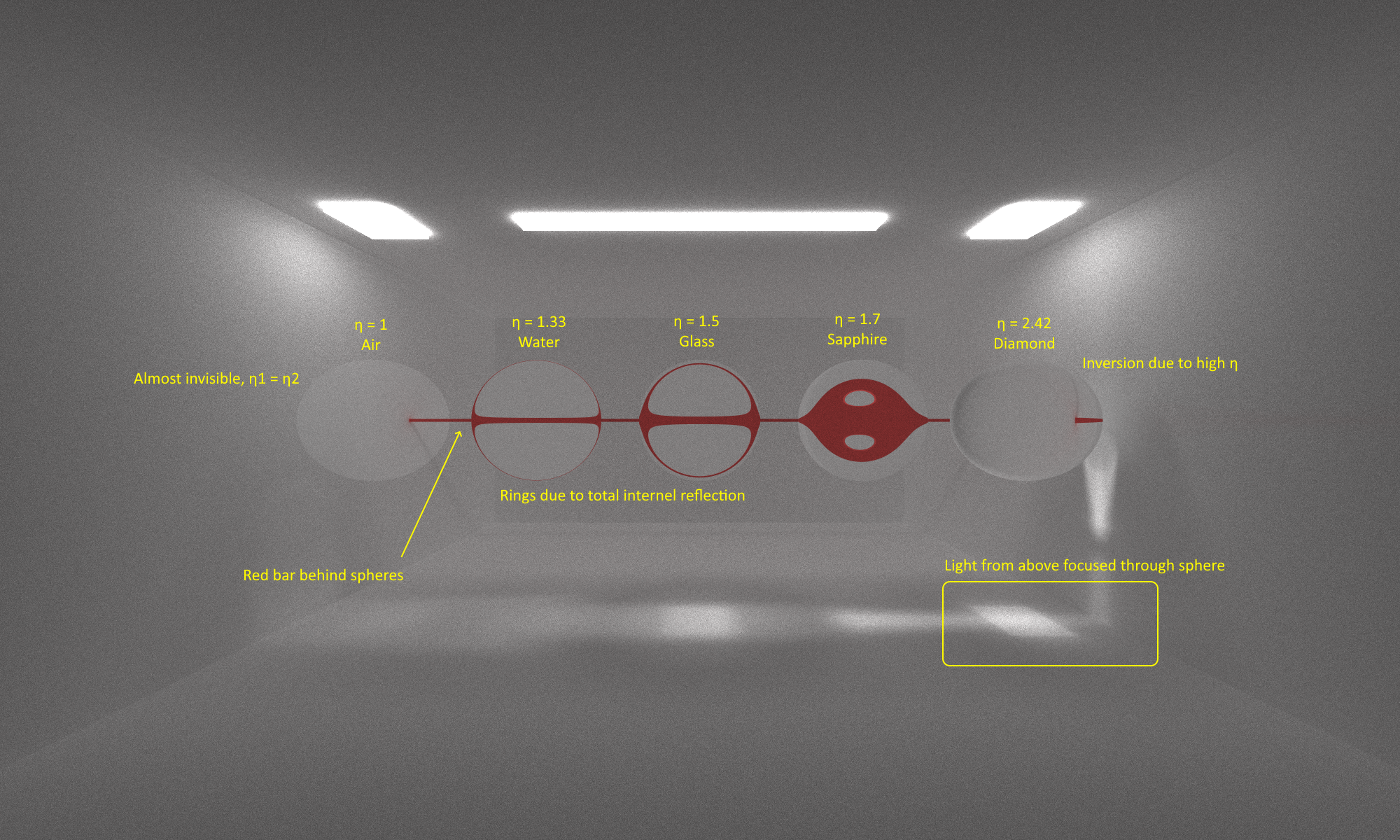
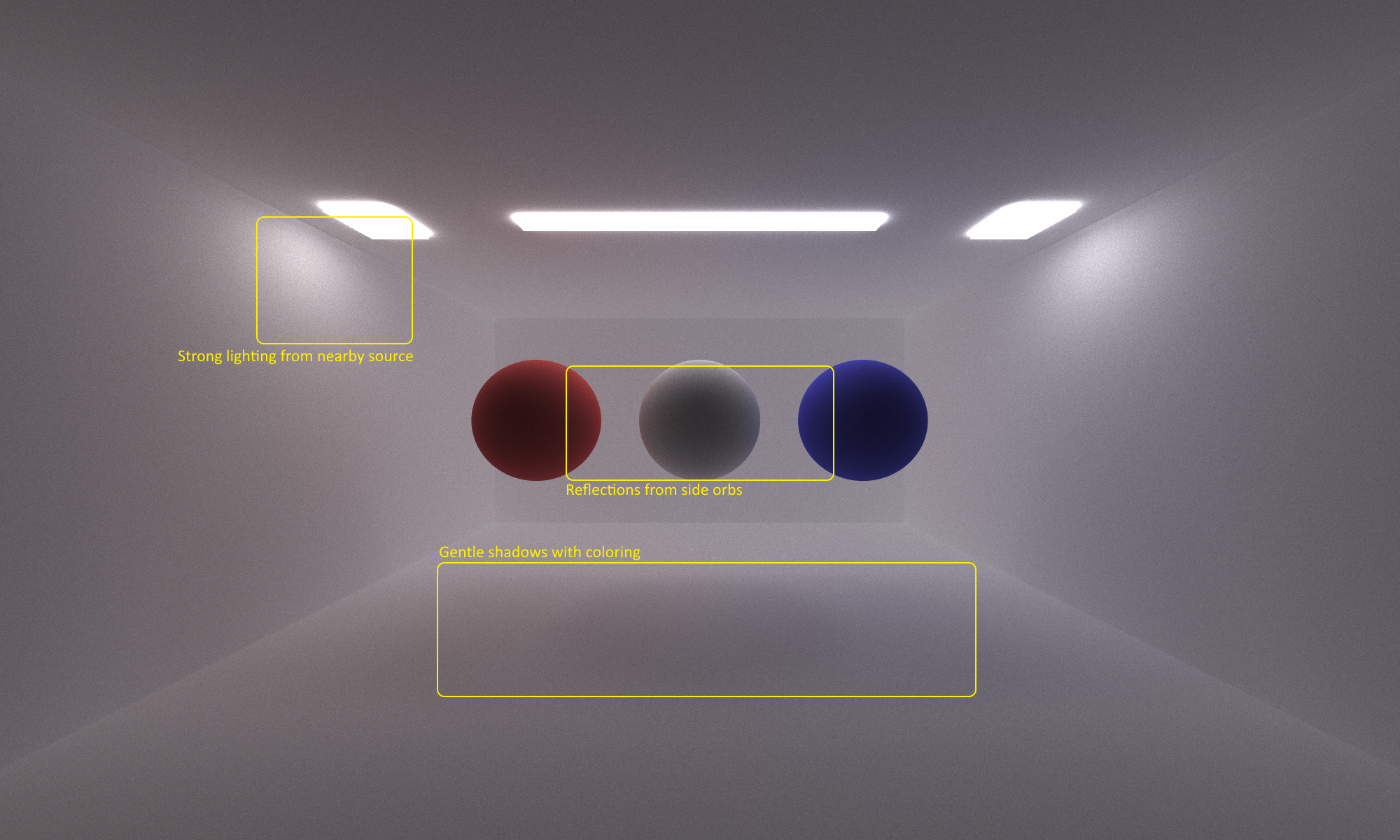
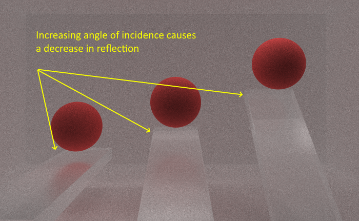
Fresnel Effect
Additionally, we must take Fresnel Effects into consideration. On a reflective/refractive surface, fresnel effects will cause reflections to appear stronger at narrower θ and weaker at wider θ. I use Shlick’s Approximation to produce a good-enough estimation on when a ray will reflect back and when it will transmit through. Note this is a different check than the critical angle.
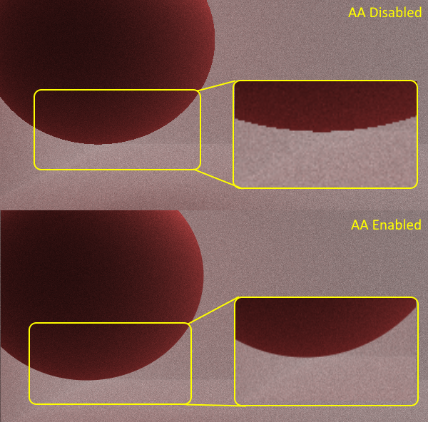
Antialiasing
Because the camera generates sample points in a regular pattern, rays will always strike the center of each pixel on the first bounce. This can lead to jagged edges on objects since the pixel is not entirely one color, but the point sampled is just one color. I implement anti-aliasing by applying a ±0.5f jitter to each ray when it is generated at the camera. This will allow our samples to randomly hit a position in the first pixel, and then these random points are samples over many iterations to produce an average of the colors in that pixel. This random sampling to produce a better average is known as stochastic sampling.
Depth of Field
In the base pathtracer, the camera is treated as a pinhole-camera. That is, all the rays begin at the same point, minus some small jitter from the Antialiasing if enabled. In a real world camera, there is a lens and a focal distance included. I simulate this in my pathtracer by projecting each sample onto a small concentric disk with lens radius r a focal distance ⨍ from the camera. This creates a depth-of-filed effect that can be controlled by modifying the two variables. Increasing the lens radius increases the blurring effect seen as objects move out of focus. Increasing the focal distance moves the focal plane back, increasing the depth of focus.
| ⨍ = 5, r = 0.01 | ⨍ = 15, r = 0.01 |
|---|---|
 |
 |
| ⨍ = 5, r = 0.05 | ⨍ = 15, r = 0.5 |
|---|---|
 |
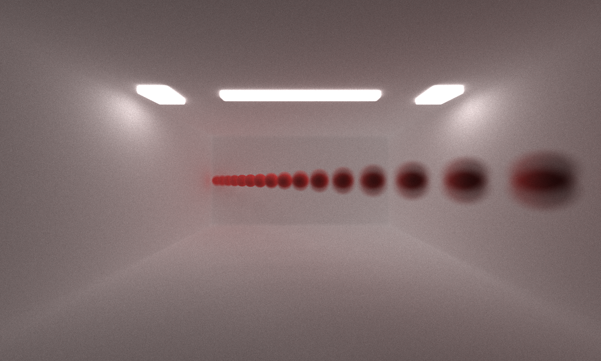 |
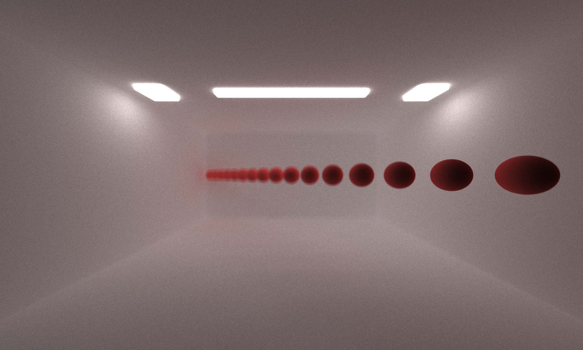
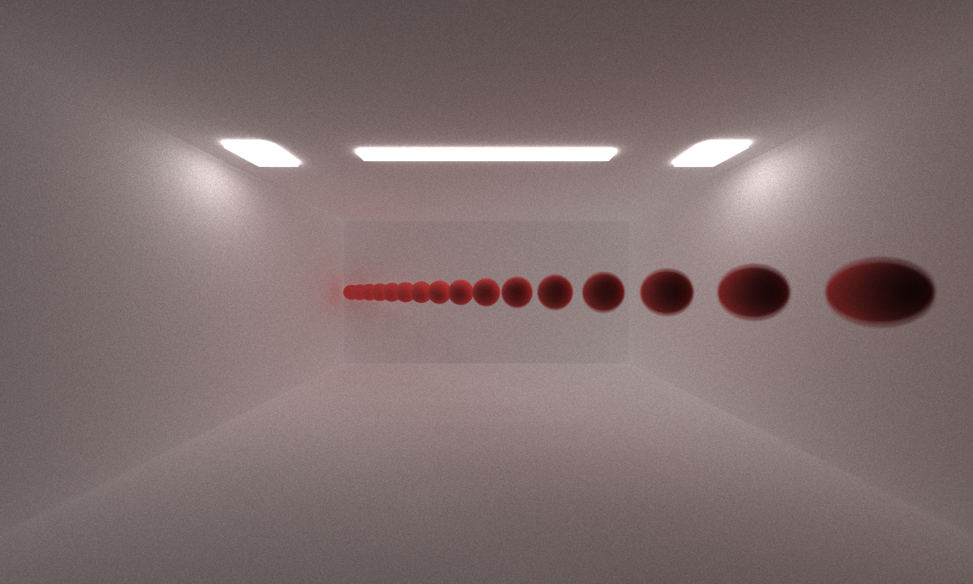
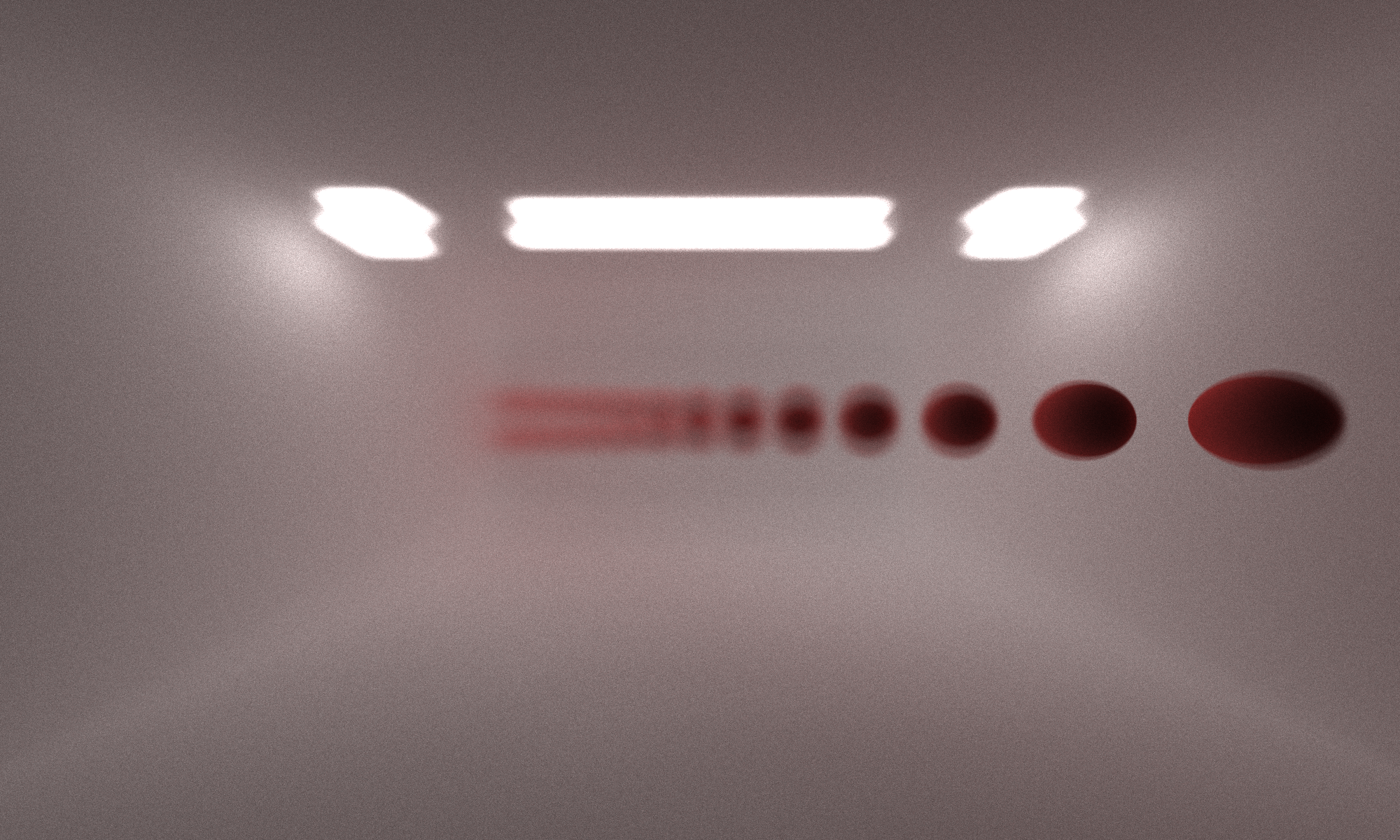
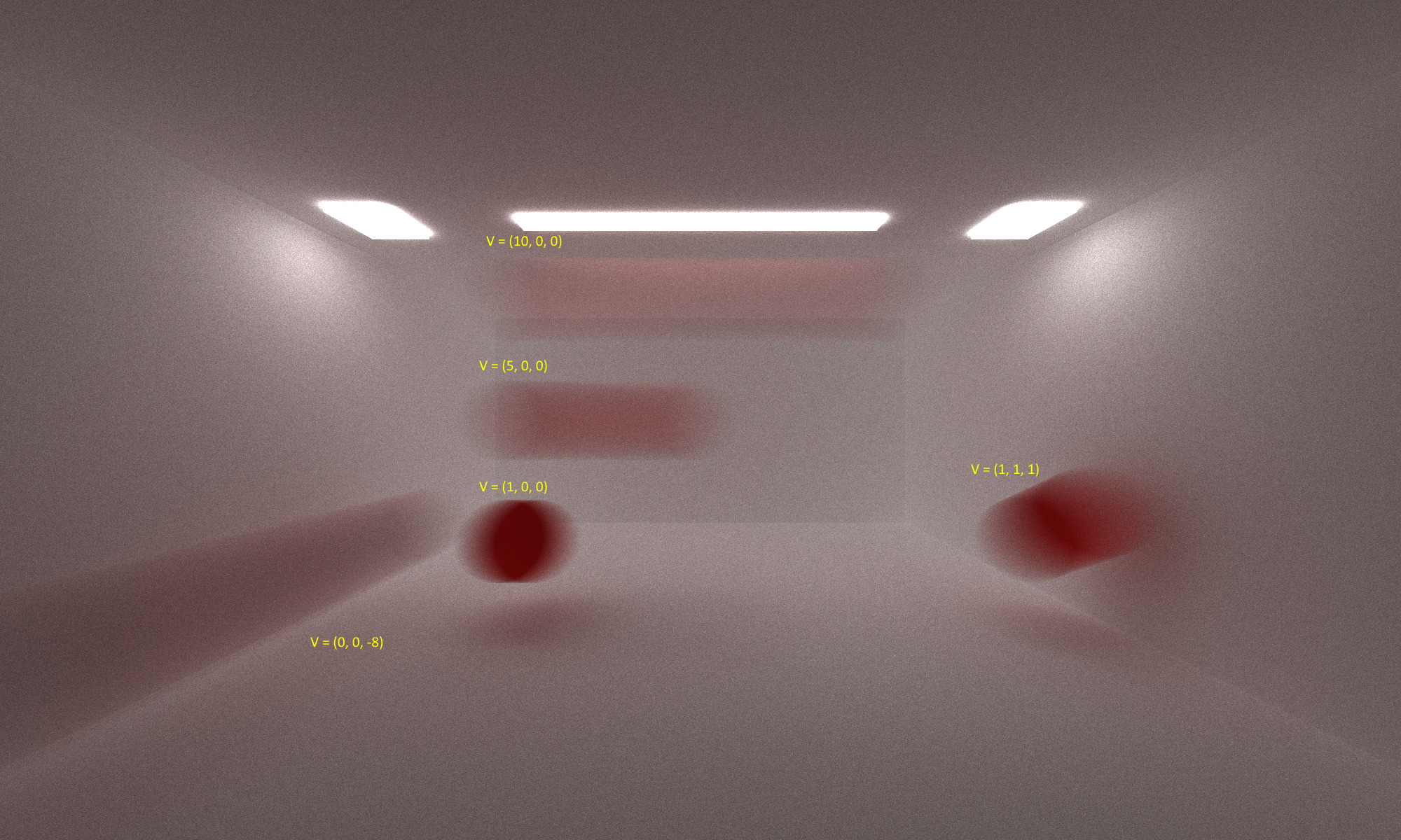
Motion Blur
A normal camera has a shutter open and a shutter close time. The final image from the camera naturally integrates over that time frame, but my renderer does not take time into account. If an object was moving in the scene, the movement would not be perceptible. I added a motion blur feature to account for this. Each object can be defined with a velocity vector in the scene description file. Each ray is then assigned a random point in time from 0 to 1. When intersections are tested, the render transforms each object by adding the displacement caused by the object velocity at that point in time. This creates a nice blurring effect, amplified by the velocity of the object.
glTF Objects
I implemented the tools needed to load glTF files and convert them into the objects used by my renderer. However, I stopped short at implementing just the physical geometries of the object and not the textures. My renderer also has lots of trouble with any complicated geometry, likely due to my intersection test having no current methods of culling objects. Overall it allows for some uninteresting objects to load. Future work would include loading textures and adding performance optimizations to allow for more interesting objects to be loaded.
Compaction of Terminated Rays
The pathtracer will fire off one ray per pixel at first, but many of those rays will terminate by falling off the scene or hitting a light source. Computing on these rays is wasteful and would lead to wasted threads in our warps and blocks. After each shading step, the device data containing all arrays is partitioned into an alive side and a terminated side. The ray buffer length is then adjusted so subsequent kernels will only operate on the living rays. This reduces the number of wasted threads per loop.
First-Bounce Caching
The camera generates rays in every direction on the first iteration, and many rays terminate after the first iteration. This leads to a very expensive first iteration normally. To help reduce the cost of this first iteration, the first set of bounces and shaders are cached by the renderer so that subsequent samples can reuse the cached first iteration data. This does not help when antialiasing is used since each first iteration is jittered randomly. Therefore, when antialiasing is enabled, the first iteration cache is disabled.
Material Sorting
To improve kernel performance, I sort the arrays used for intersections by the material ID. This helps by reducing the largest divergence split in the shaders. When the shader starts, it looks at the properties of the material and then choses a distribution function based on that. If a diffuse material, reflective material, and refractive material are all in the same warp, this leads to horrendous performance. Each kernel will diverge in the early stages of the shader and each will have to perform serially. By grouping materials together, divergence is limited to instances where the angle of incidence causes some unique behavior in each kernel.
Performance Comparison
Combining the above three optimizations, I generated a scene of 2000 random spheres bounded in a room. I also calculated 200 unique materials randomly distributed between the spheres. I then ran each 5 scenarios under different configurations to collect my data, measuring the elapsed milliseconds for each iteration of the CUDA renderer. The chart below contains average values for each iteration across 200 samples. I excluded the first iteration of the Pathtracer to show the advantage of the First-Bounce caching optimization.
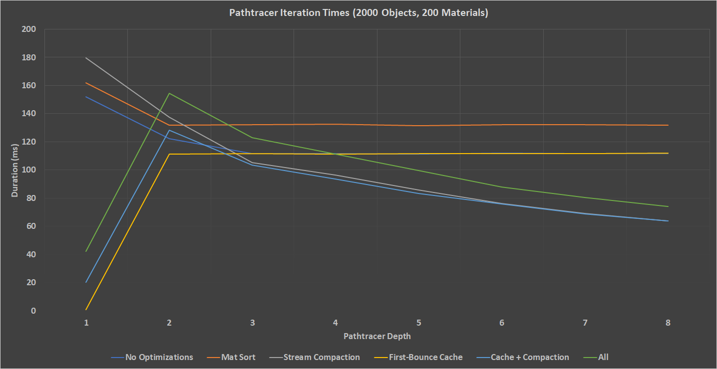
Running with no optimizations provides a solid baseline to the Pathtracer. The first iteration takes significantly longer to calculate for all modes due to every ray being shaded. Many rays will fall off the scene and terminate after the first iteration. If we look at the material sort data, the performance is actually worse. Compared to the base Pathtracer, the Material Sort has a 14% decrease in performance. The goal of material sorting is to keep similar materials close in memory to improve cache coherency and reduce high-cost memory calls to global memory. However, with 200 materials, the cost of sorting the materials buffer is significant (16ms added). If we factor our the additional 16ms per depth in the material sort optimization, the result is about equal to having no optimizations. Rerunning the test with only two materials showed no improvement to the algorithm. This tells me that the cost of reading material data is insignificant compared to the costs of computing the shader. As we’ll also see in the All optimization, the Material Sort optimization only serves to add 14-16ms per loop to the pathtracer.
| Material Sorting Performance| | —- |
| Num. Materials | Avg. Duration |
|---|---|
| 200 | 133.4 ms |
| 2 | 136.4 ms |
More interesting are the Stream Compaction and First-Bounce Cache optimizations. When only Stream-Compaction is enabled, we can see that there is a 65% increase in performance from the Depth 1 to Depth 8. This makes sense, since each loop requires less CUDA kernels to execute.
| Ray Reduction Using Stream Compaction| | —- |
| Depth | Active Rays | % of Total |
|---|---|---|
| 0 | 2400000 | 100.00% |
| 1 | 2392104 | 99.67% |
| 2 | 1895971 | 79.00% |
| 3 | 1715007 | 71.46% |
| 4 | 1523808 | 63.49% |
| 5 | 1382218 | 57.59% |
| 6 | 1253035 | 52.21% |
| 7 | 1144541 | 47.69% |
| 8 | 0 | 0% |
The First-Bounce cache optimization similarly adds a huge benefit by not having to repeat the most costly iteration. Referring to the Ray Reduction table, we can see that by caching the first set of ray intersections, we avoid having to calculate intersections of 20% of the rays. By combining the First-Bounce cache and Stream Compaction optimizations, we can achieve the highest performance. However, there are many other optimizations that can be made to the pathtracer. Breaking the shader kernel down into smaller pieces can reduce divergence, especially when dealing with paths depending on random variations in reflection/refraction. It might be work sacrificing some randomness to keep all the threads in a warp in step with one another.
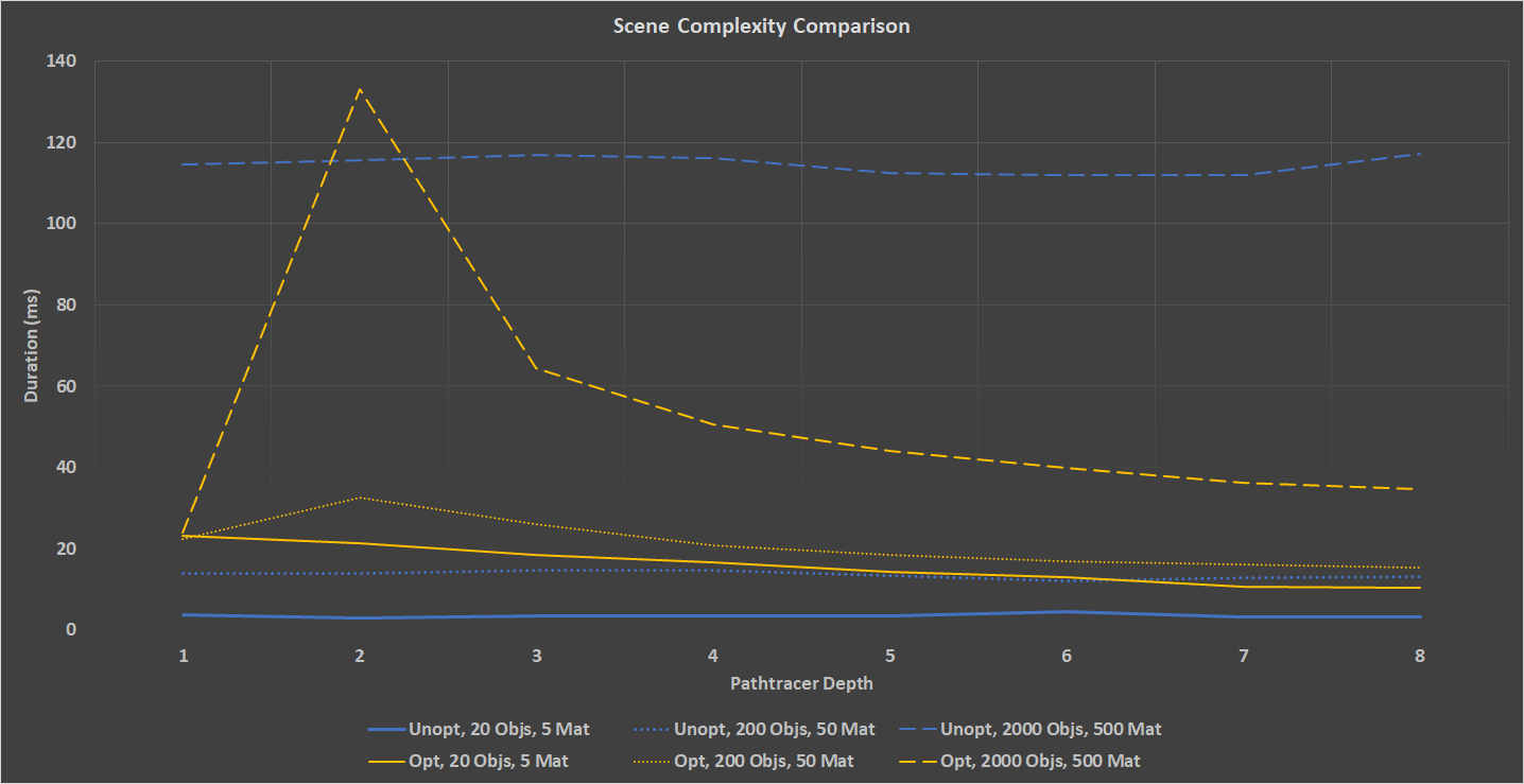
It is also interesting to see the performance difference between the optimized and unoptimized pathtracer with different scene complexities. I ran both optimized and unoptimized pathtracers through 3 scenes: 20 objects, 200 objects, and 2000 objects. The unoptimized pathtracer did significantly better in simple cases, but as the number of objects went up, the better the optimized pathtracer performed. There is a spike in duration for the optimized pathtracer in the second depth. This was measured and attributed to the extra work done to perform stream compaction on the second set of rays. After this initial spike the performance improves greatly. In the most complex scene, the unoptimized pathtracer takes 916ms per iteration, while the optimized pathtracer needs only 426ms.
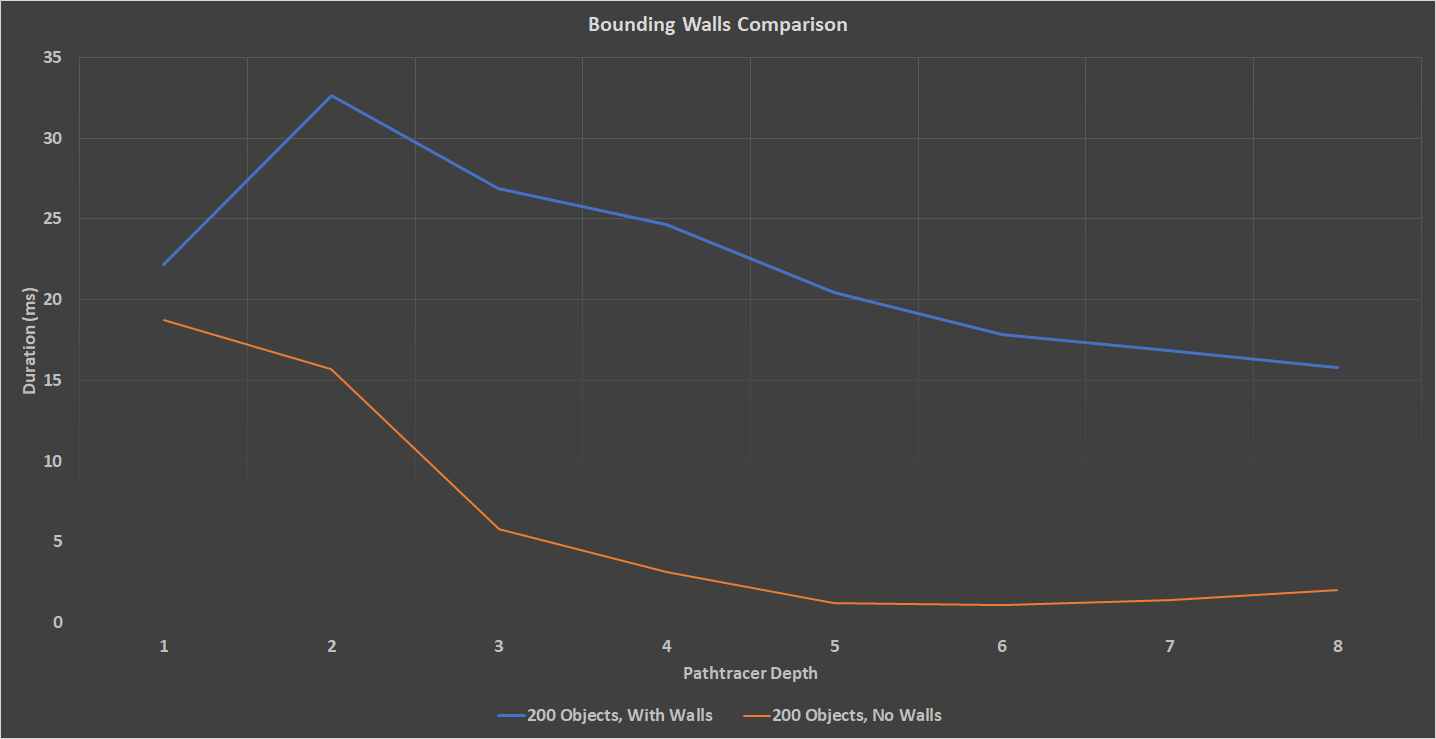
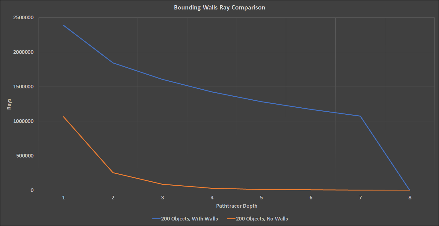
Lastly, I ran a comparison with a 200-Object scene with bounding walls and a scene with no walls. As was expected, the scene with no walls performed much better. This is due to the huge number pf rays that become irrelevant after even the first iteration. As can be seen in the charts below, the scene with no bounding walls loses 76% of its rays after the first bounce, while the bounded scene only loses 22% of its rays. By the end of the iteration, the bounded scene still has 44% of its rays, while the unbounded scene has 0.3%.
Bloopers
Lets laugh with me, not at me.
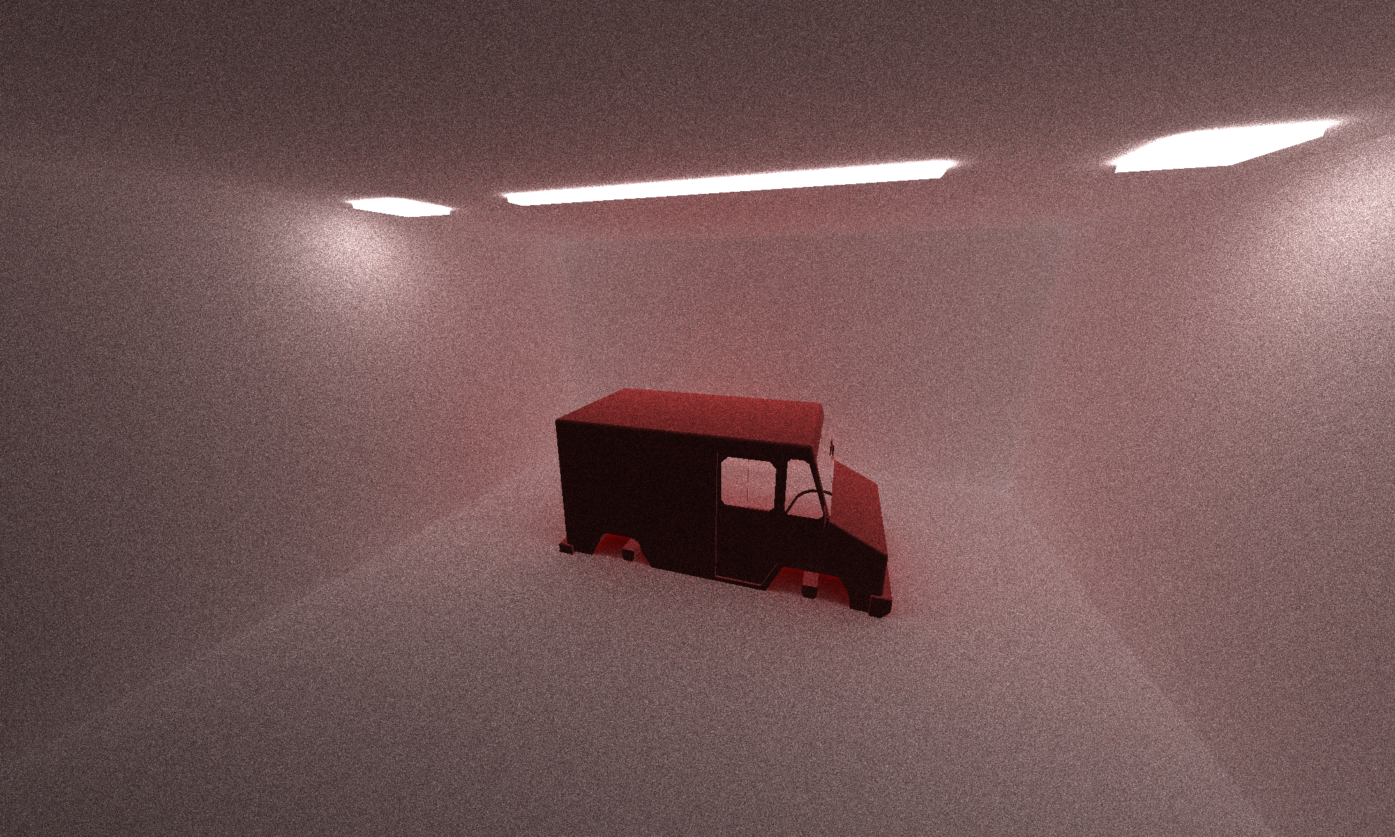
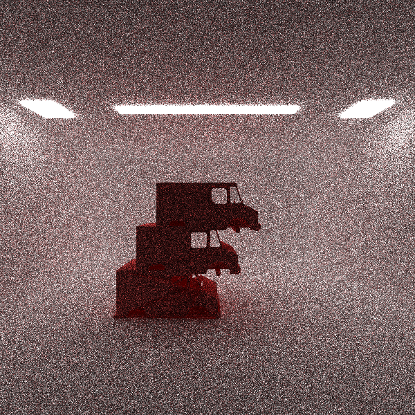
Sometimes you’re driving your milk truck and you just start to disassociate from the mortal plane.
While working on the DOF, I was not transforming the right coordinates and the pathtracer decided to knock my camera to the ground.
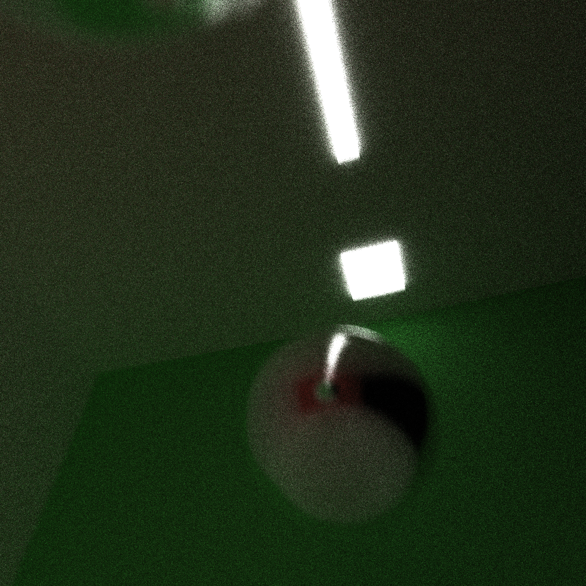
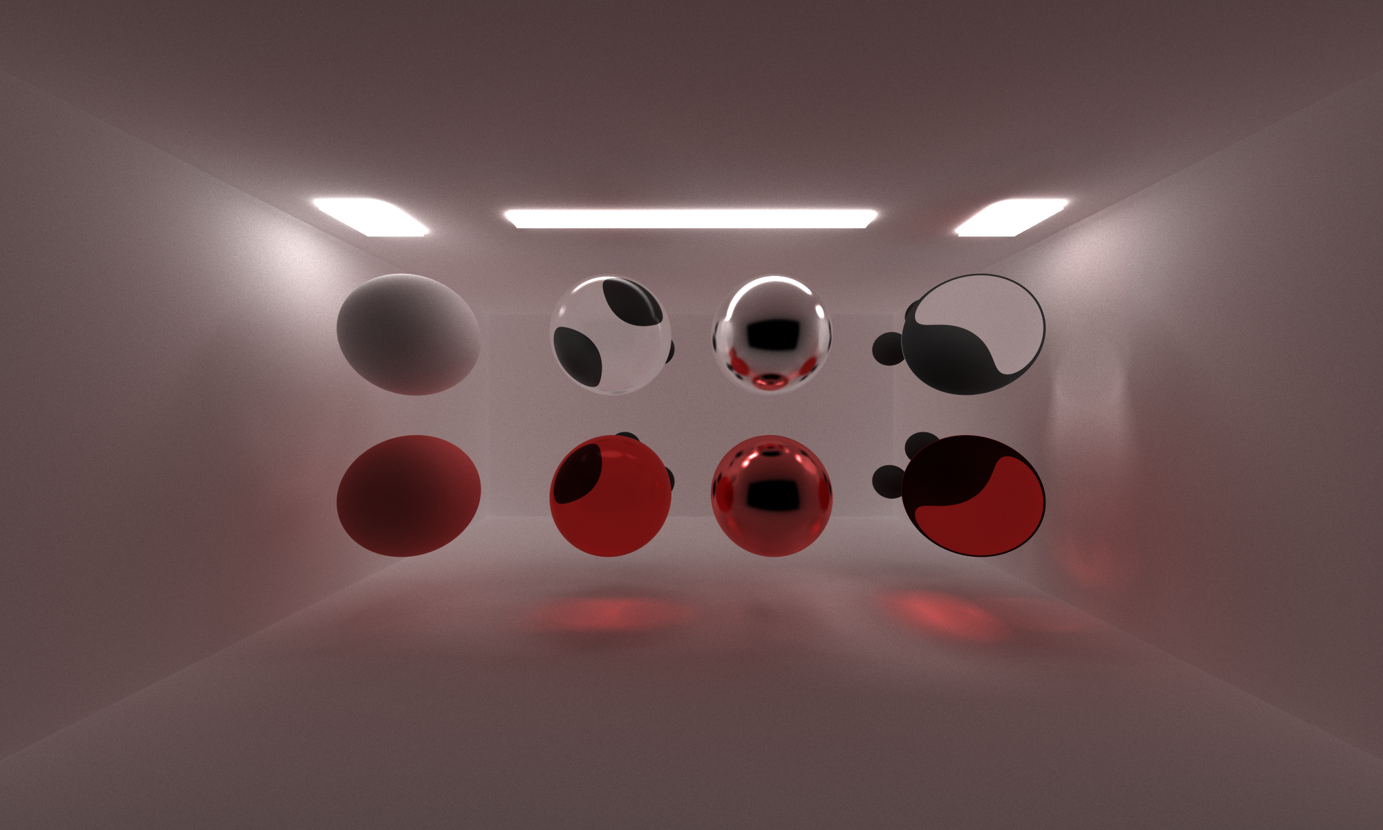
And lastly, the most frustrating bug. When calculating the new origin after a ray intersects another object, it is useful to bump the origin away from the actual intersection. This is done to tell the pathtracer that the ray has truly left the intersection. If the origin is not offset enough, the ray will bounce in an object for eternity. That is what was happening when I tried to calculate refraction. I ended up with some cool, cloudy balls, but it was, overall, a big use of my time.
Acknowledgements
Physically Based Rendering, Third Edition: From Theory To Implementation
PBRT3 was seriously the most useful resource I found. Many of my implementation details came from this work.
Another excellent resource, especially for understanding some of the complicated math behind these functions.
Library used for loading gltf files into my renderer. Also used some example code to speed up implementation.